4.8 Fluid Dynamics: Integration-Custom
1. Import CAD
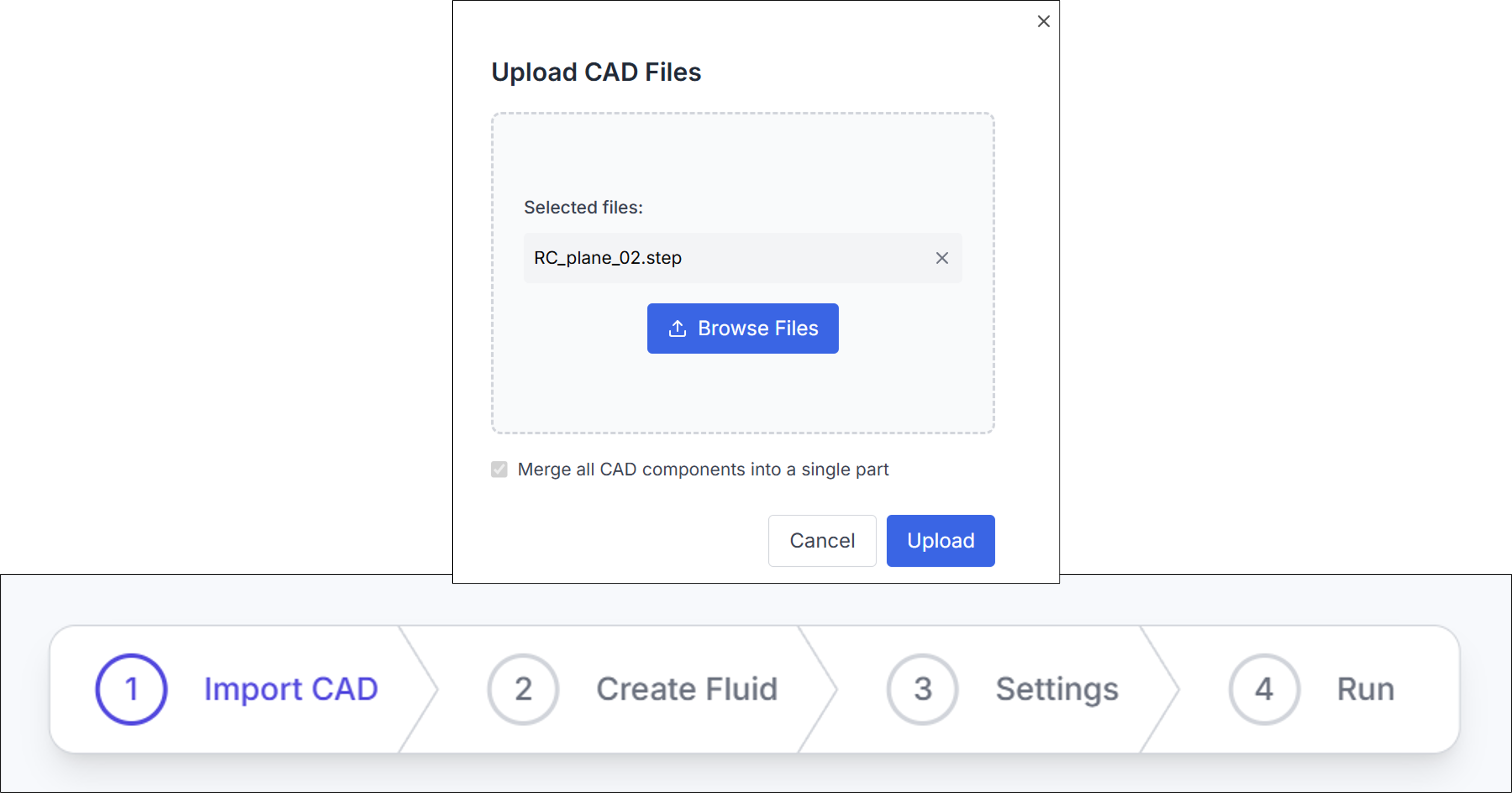
In the Integration-Custom process, it is assumed that the user has a CAD file with the .step extension. Select the desired file using the Browse Files button, then proceed with Upload.
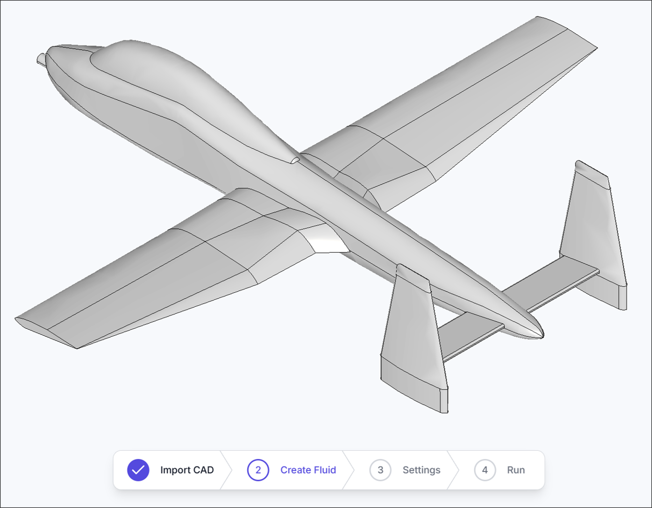
After uploading, verify that the CAD file has been successfully recognized.
2. Create Fluid
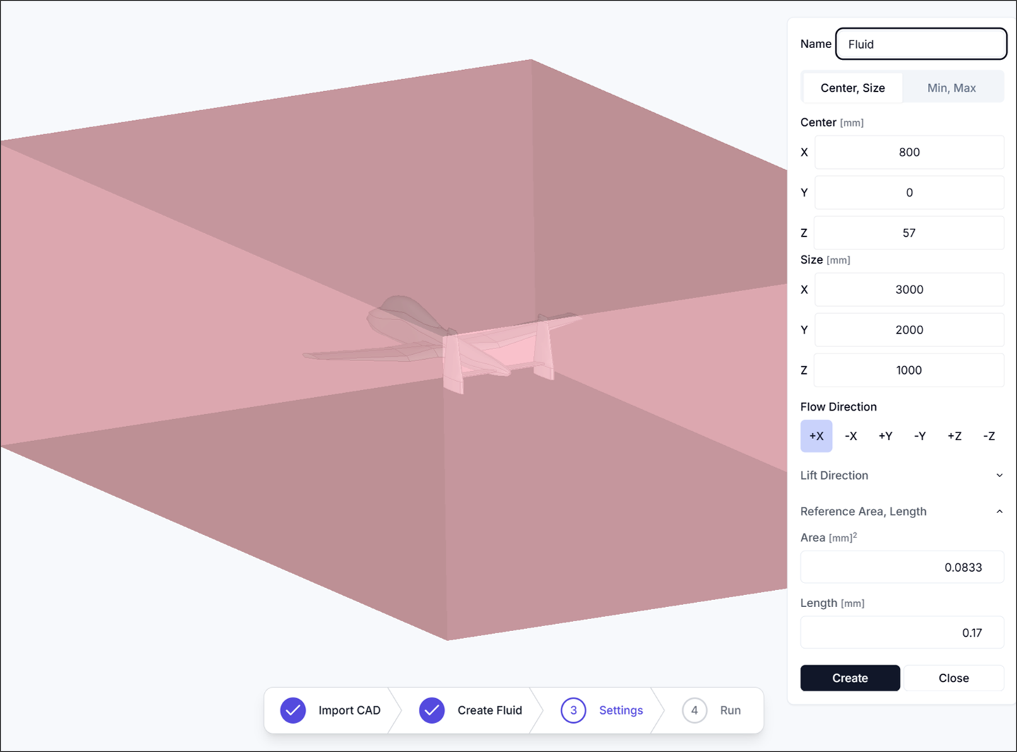
The Create Fluid process defines the fluid region for the simulation.
When setting the Flow Direction, note that the axis is aligned with the aircraft’s forward direction, but the direction itself is reversed to represent the incoming airflow.
- Center: Set the center of the fluid domain as
<x, y, z>. - Size: Set the size of the fluid domain as
<x, y, z>. - Flow Direction: Define the direction of the incoming flow.
- Lift Direction: Set the direction of lift, typically perpendicular to the upper surface of the main wing.
- Reference Area: Specify the reference area, usually based on the main wing’s planform area.
- Reference Length: Specify the reference length, typically the Mean Aerodynamic Chord (MAC).
Mean Aerodynamic Chord (MAC):
A reference length used in aerodynamics, particularly for defining characteristics of an aircraft wing.
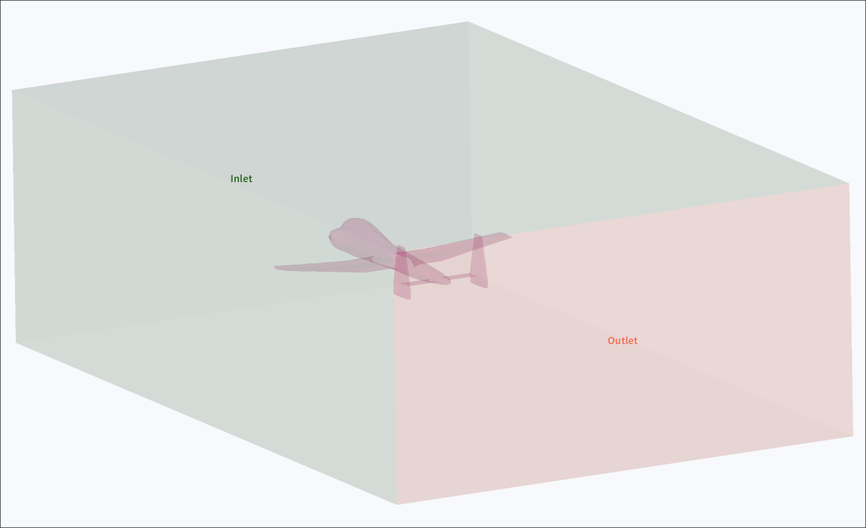
After creating fluid, verify that the fluid region has been successfully generated.
3. Settings
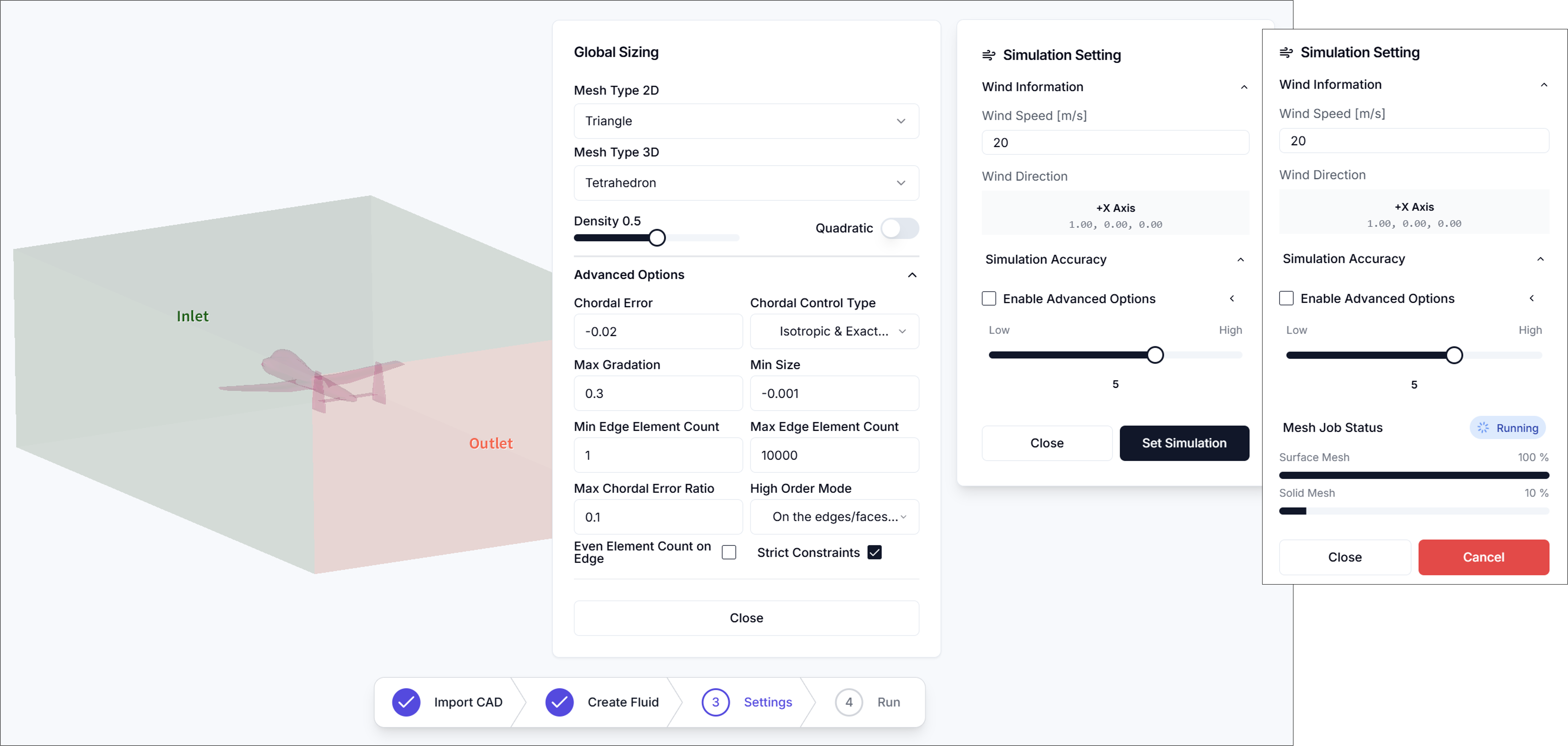
The Simulation Settings process is used to define wind information and generate the mesh.
3.1. Wind Information
-
Wind Speed [m/s]: Define the wind velocity.
-
Wind Direction: Indicates the wind direction as defined in the Create Fluid step.
3.2. Simulation Accuracy
The mesh resolution can be adjusted to suit the desired level of detail.
Detailed configuration options are described below.
Meshing Parameters (Advanced Options)
-
Enable Advanced Options: Enables access to detailed meshing configuration.
-
Mesh Type 2D
Selects the type of surface mesh applied to faces.
- Triangle
- QuadDominant
- Quadrangle
-
Mesh Type 3D
Selects the type of volume mesh used within the fluid domain.
- Tetrahedron
- HexaDominant
- Hexahedron
-
Density
Controls the overall mesh density using a normalized slider. Higher values produce finer meshes.
-
Chordal Error
Defines the maximum allowable deviation between the mesh edge and the actual geometry. A lower value results in higher surface fidelity.
-
Chordal Control Type
Determines how the chordal error is applied.
- No Curvature
- Isotropic & Approximate Curvature
- Anisotropic & Approximate Curvature
- Isotropic & Exact Curvature
- Anisotropic & Exact Curvature
-
Max Gradation
Specifies the maximum allowed ratio between adjacent element sizes to control smoothness in mesh transitions.
-
Min Size
Sets the minimum edge length allowed in the generated mesh.
-
Min Edge Element Count
Defines the minimum number of elements along an edge.
-
Max Edge Element Count
Defines the maximum number of elements allowed along an edge.
-
Max Chordal Error Ratio
Sets the maximum ratio between actual chordal error and the user-defined target value.
-
High Order Mode
Determines how high-order elements (for curved surfaces) are treated.
- Interpolated
- On the edges/faces but not equidistant
- On the edges/faces but equidistant
-
Even Element Count on Edge Enforces an even number of elements on edges for better symmetry or periodicity, if applicable.
Once all parameters are properly configured, click Set Simulation to generate the mesh.
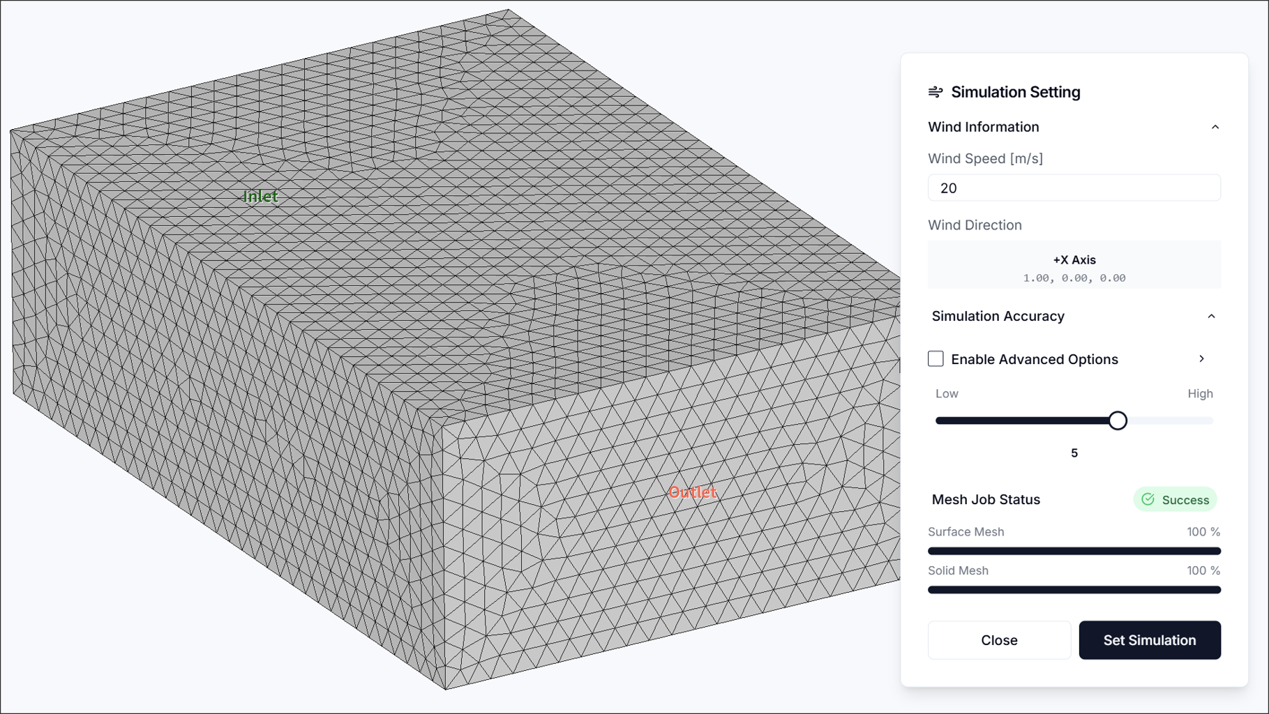
Finally, Ensure the generated mesh to ensure it is appropriate for the simulation.
4. Run Simulation
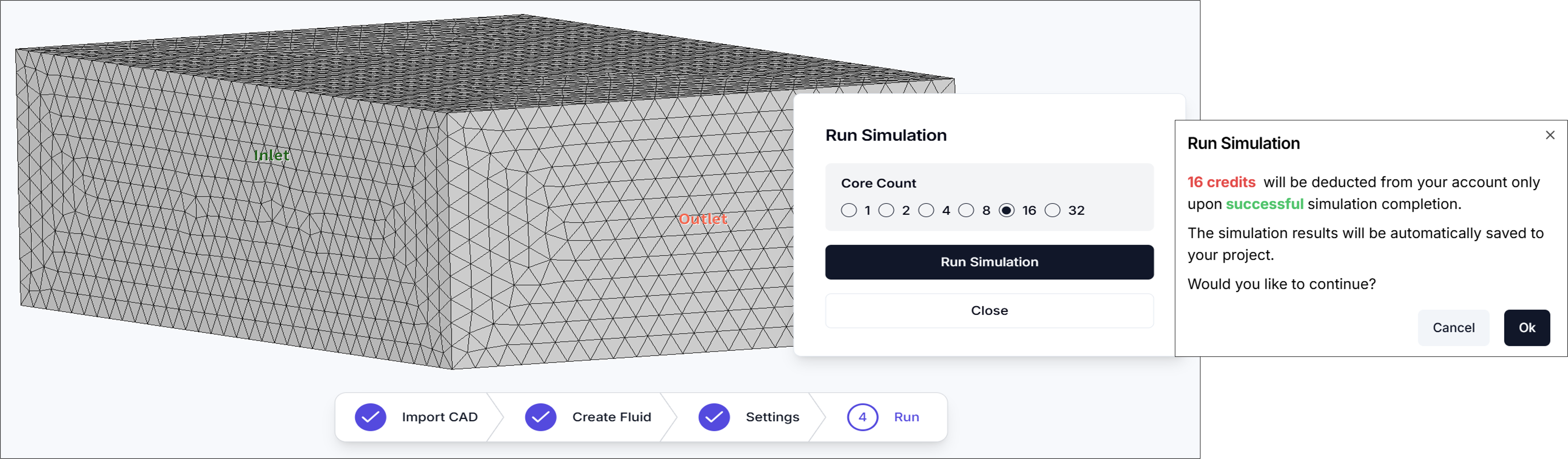
In the Run Simulation step, specify the Core Count and start the analysis.
In general, increasing the core count reduces simulation time.
However, using more cores will consume more credits.
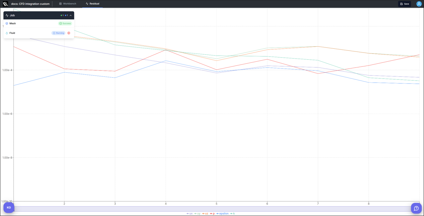
Once the simulation starts successfully, the interface will automatically switch to the Residuals window.
Residual
A fundamental indicator used to evaluate the convergence of a flow simulation.
To determine whether the simulation has converged properly, the residual values of each solution variable must be sufficiently low.
5. Results
Once the simulation is completed, the Result and Report windows will become available.
5.1. Result(3D contour)
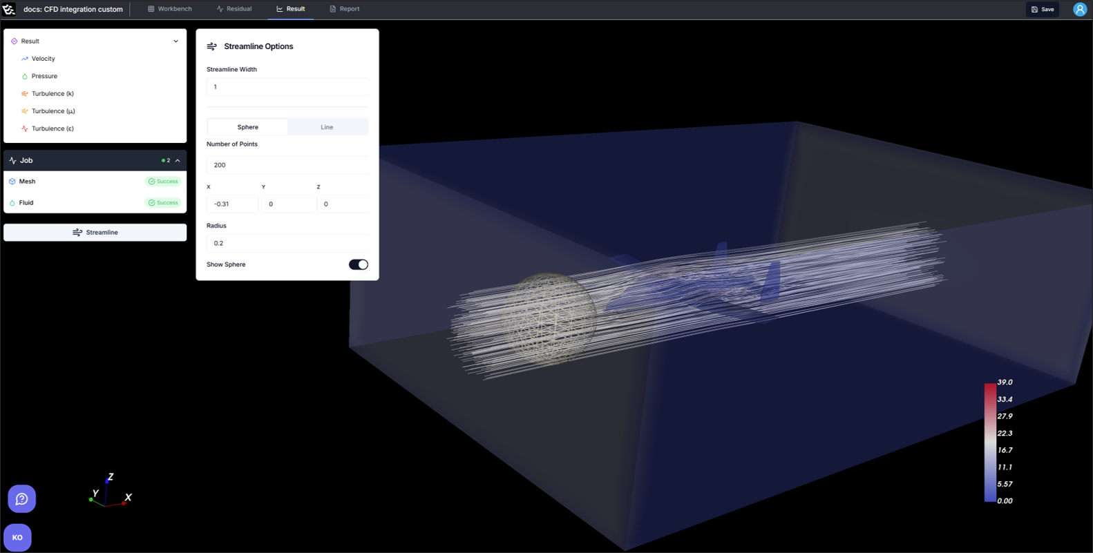
The Result window provides visual representations of various physical fields.
- Velocity
- Streamline: Visualizes the flow of air by generating streamlines. The generation method can be selected as either Sphere or Line.
- Pressure
- Turbulence
5.2. Report
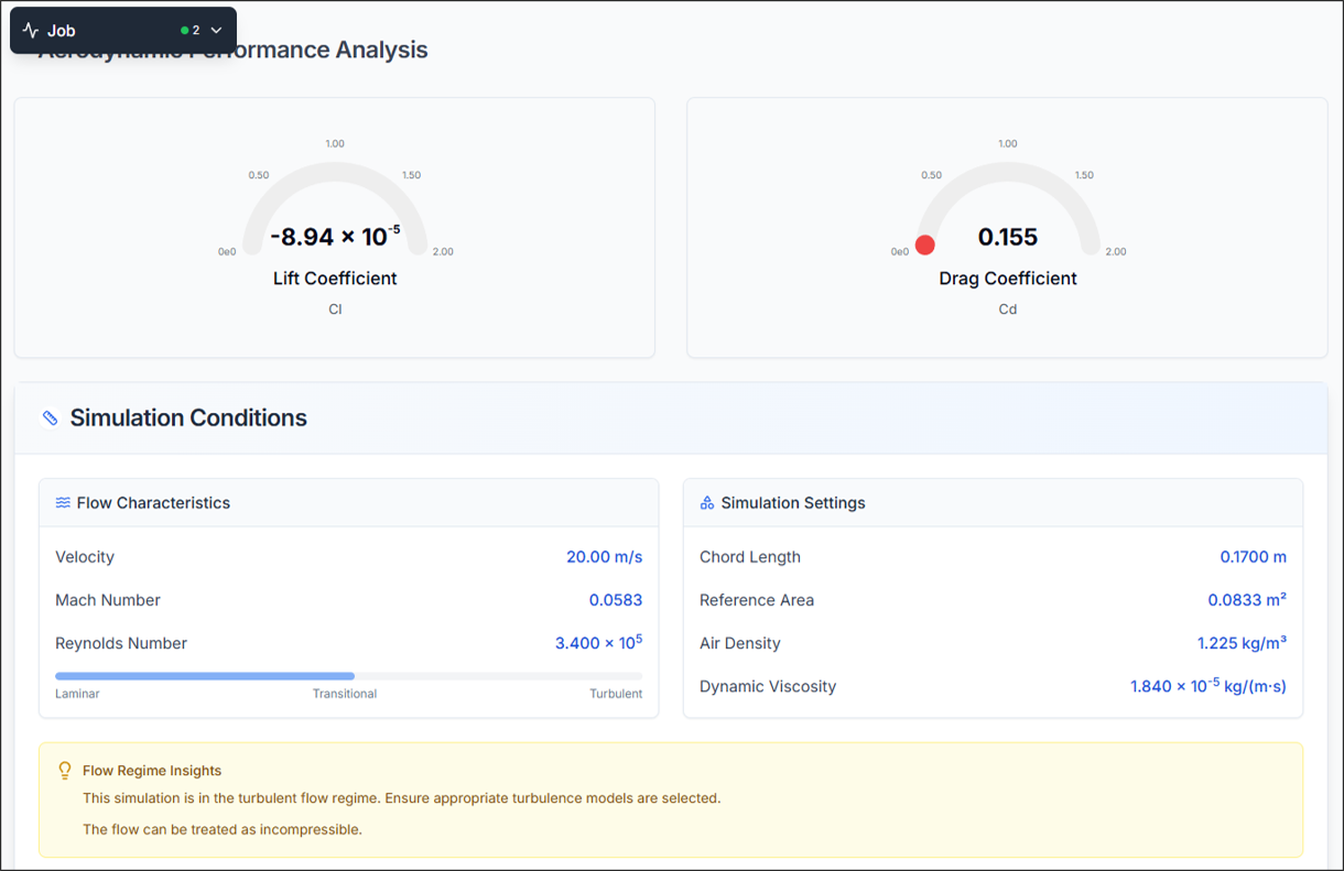
5.2.1. Aerodynamic Performance Analysis
Lift Coefficient (CL)
The Lift Coefficient is a dimensionless number that represents the lift force generated by the aircraft. It is defined by the following equation:
Where:
- : Lift force
- : Air density (typically assumed to be 1.225 [kg/m³])
- : Wind speed
- : Reference area (e.g., main wing area)
Drag Coefficient (CD)
The Drag Coefficient is a dimensionless number that represents the drag force acting on the aircraft. It is defined by the following equation:
Where:
- : Drag force
- : Air density
- : Wind speed
- : Reference area (e.g., main wing area)
Flow Characteristics
- Velocity: Equivalent to wind speed.
- Mach Number: A dimensionless quantity representing the ratio of the object's speed to the speed of sound in the surrounding medium.
- Reynolds Number: A dimensionless number representing the ratio of inertial forces to viscous forces in the fluid.
Additional Parameters
- Chord Length: Same as the Mean Aerodynamic Chord (MAC).
- Reference Area: Same as the reference area defined in the Create Fluid step.
- Air Density: Air density, generally assumed to be 1.225 [kg/m³].
- Dynamic Viscosity: A measure of a fluid's resistance to flow under an external force.
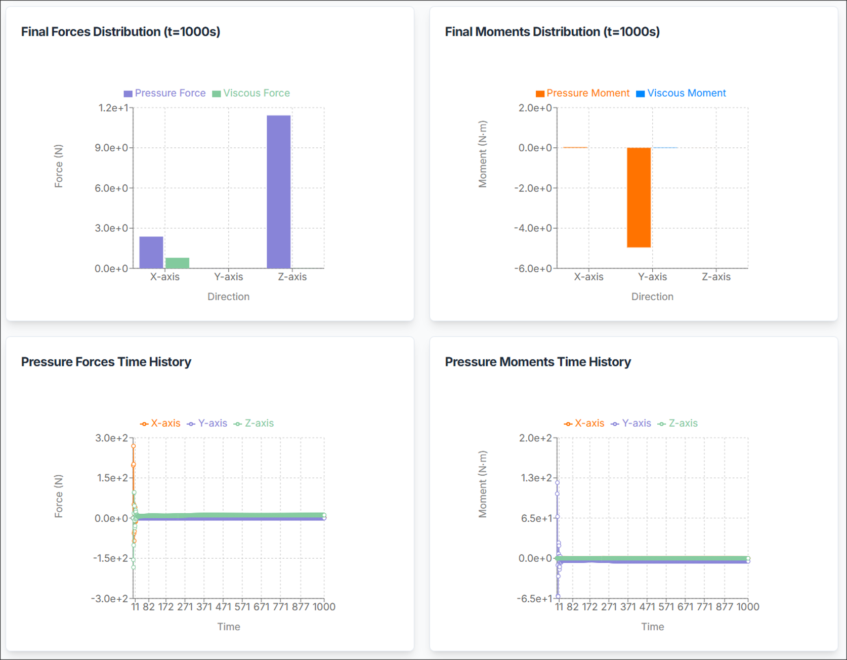
-
Force/Moments Distribution: Displays the distribution of forces and moments at the end of the simulation. The values are classified into pressure and viscous (frictional) components.
-
Time History: Shows the variation of force and moment values over simulation time. This provides insight into the convergence and temporal behavior of the aerodynamic forces and moments.
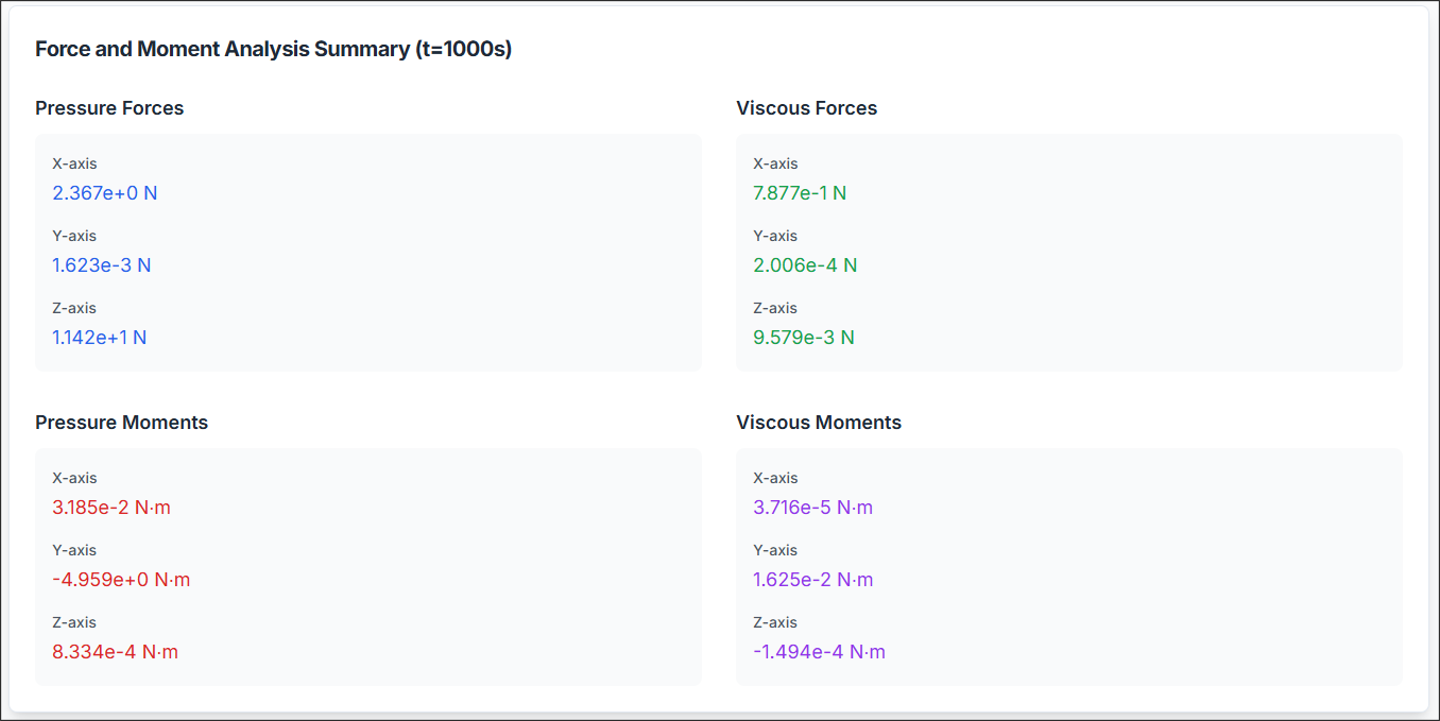
Forces and Moment Analysis Summary
Provides a numerical summary of the final force and moment values, categorized into contributions from pressure and viscous forces based on the state at the end of the simulation.
Need Assistance or Have Questions?
Frequently Asked Questions: FAQ Link
Support Inquiries: support@everysim.io